Plant Disease Detection using Machine Learning with Source Code

Ensuring that crops are healthy and full of nutrients is very important for long-term food production. However, diseases that affect plant leaves can slow growth and yield, a problem for farms worldwide. Conventional methods for finding diseases often involve inspecting things by hand, which can take a long time and lead to mistakes. Here comes machine learning, which has changed the game in agriculture by creating new ways to quickly and correctly find leaf diseases.

Understanding Leaf Diseases

Before getting into the details of machine learning-based detection, it’s important to understand the basics of leaf diseases. These diseases include a variety of fungal, bacterial, and viral infections, as well as physiological defects, all of which cause unique symptoms on the leaves of plants. From white mold to bacterial disease, each disease has a distinct appearance, making early detection difficult for farmers.

The Limitations of Traditional Methods

In the past, farmers had to look at leaves by hand to find leaf diseases. This method worked to some extent, but it takes a lot of work and is easy to overlook. Also, how different people see things can make diagnoses inconsistent. More effective ways to find diseases are needed because farming areas are growing, and diseases are becoming more complicated.

Enter Machine Learning

Traditional methods of finding diseases have drawbacks that machine learning systems could help fix. These algorithms can accurately tell the difference between different signs by using huge datasets containing images of healthy and sick leaves. Machine learning models can quickly find signs of disease through pattern recognition and classification, which lets people take action before they get infected.

Training the Algorithm

The functioning of machine learning-based detection systems depends on the algorithm’s training. This involves adding labelled images of healthy and diseased leaves into the model, allowing it to gain knowledge of each state’s unique characteristics. With increased data analysis iteration, the algorithm shows enhanced precision in classifying leaves images, which creates a foundation for strong disease detection.

Image Preprocessing Techniques

Preprocessing techniques extract important information and improve image quality before feeding the images into the machine-learning model. Resizing, normalization, and augmentation are a few strategies used to standardize the input data and enhance the algorithm’s performance. The dataset is refined through preprocessing so that the model can concentrate on identifying significant patterns in the images.

Real-Time Detection and Monitoring

The best thing about plant disease detection using machine learning is that it can monitor crop health in real-time. With sensors and recording devices built in, these systems can constantly look over fields for signs of disease and inform farmers immediately about any possible threats. This proactive method allows people to step in quickly, reducing crop losses and increasing yields.

Scalability and Adaptability

Another significant advantage of machine learning in agriculture is its scalability and adaptation across different crops and conditions. Like previous approaches, which may be limited to certain diseases or plant species, machine learning algorithms can be trained to detect a wide range of leaf diseases. Furthermore, these models can adjust to changing disease patterns, ensuring their value in dynamic agricultural settings.

Challenges and Considerations

Even though machine learning has a lot of potential for detecting leaf diseases, there are certain difficulties. Some aspects that need to be carefully considered are data availability, model interpretability, and implementation costs. Another major challenge is guaranteeing the algorithms’ durability and generalizability under various growing situations.

Plant Disease Detection Source Code

To create a plant disease detection in Python. First, download the dataset from here and then follow these steps:

1. Importing Libraries

The required libraries, including matplotlib, torch, torchvision, pandas, and numpy, are imported into this block. Additionally, it imports particular modules from torchvision, including the SubsetRandomSampler from torch.utils.data.sampler and datasets, transformations, models, nn, and functional.

				import numpy as np
import pandas as pd
import matplotlib.pyplot as plt
import torch
from torchvision import datasets, transforms, models
from torch.utils.data.sampler import SubsetRandomSampler
import torch.nn as nn
import torch.nn.functional as F
from datetime import datetime

import numpy as np
import pandas as pd
import matplotlib.pyplot as plt
import torch
from torchvision import datasets, transforms, models
from torch.utils.data.sampler import SubsetRandomSampler
import torch.nn as nn
import torch.nn.functional as F
from datetime import datetime

2. Defining Image Transformations

This block defines a set of image preprocessing transformations that use torchvision transforms. Compose. These changes include scaling, center cropping, and turning photos into tensors.

				transform = transforms.Compose(
    [transforms.Resize(255), transforms.CenterCrop(224), transforms.ToTensor()]
)

transform = transforms.Compose(
    [transforms.Resize(255), transforms.CenterCrop(224), transforms.ToTensor()]
)

3. Loading Dataset

This block loads images from a folder (“dataset_images”) using torchvision’s datasets.ImageFolder and applies the defined transformations.

				dataset = datasets.ImageFolder("dataset_images", transform=transform)

dataset = datasets.ImageFolder("dataset_images", transform=transform)

4.Splitting Dataset Indices

This block randomly shuffles the indices of the dataset and splits them into train, validation, and test indices based on predefined proportions.

				indices = list(range(len(dataset)))
split = int(np.floor(0.85 * len(dataset)))
validation = int(np.floor(0.70 * split))

train_indices, validation_indices, test_indices = (
    indices[:validation],
    indices[validation:split],
    indices[split:],
)

indices = list(range(len(dataset)))
split = int(np.floor(0.85 * len(dataset)))
validation = int(np.floor(0.70 * split))

train_indices, validation_indices, test_indices = (
    indices[:validation],
    indices[validation:split],
    indices[split:],
)

5. Defining Model Architecture

This block defines a CNN class inheriting from nn.Module, specifying the architecture with convolutional and dense layers.

				class CNN(nn.Module):
    def __init__(self, K):
        super(CNN, self).__init__()
        self.conv_layers = nn.Sequential(
            # conv1
            nn.Conv2d(in_channels=3, out_channels=32, kernel_size=3, padding=1),
            nn.ReLU(),
            nn.BatchNorm2d(32),
            nn.Conv2d(in_channels=32, out_channels=32, kernel_size=3, padding=1),
            nn.ReLU(),
            nn.BatchNorm2d(32),
            nn.MaxPool2d(2),
            # conv2
            nn.Conv2d(in_channels=32, out_channels=64, kernel_size=3, padding=1),
            nn.ReLU(),
            nn.BatchNorm2d(64),
            nn.Conv2d(in_channels=64, out_channels=64, kernel_size=3, padding=1),
            nn.ReLU(),
            nn.BatchNorm2d(64),
            nn.MaxPool2d(2),
            # conv3
            nn.Conv2d(in_channels=64, out_channels=128, kernel_size=3, padding=1),
            nn.ReLU(),
            nn.BatchNorm2d(128),
            nn.Conv2d(in_channels=128, out_channels=128, kernel_size=3, padding=1),
            nn.ReLU(),
            nn.BatchNorm2d(128),
            nn.MaxPool2d(2),
            # conv4
            nn.Conv2d(in_channels=128, out_channels=256, kernel_size=3, padding=1),
            nn.ReLU(),
            nn.BatchNorm2d(256),
            nn.Conv2d(in_channels=256, out_channels=256, kernel_size=3, padding=1),
            nn.ReLU(),
            nn.BatchNorm2d(256),
            nn.MaxPool2d(2),
        )

        self.dense_layers = nn.Sequential(
            nn.Dropout(0.4),
            nn.Linear(50176, 1024),
            nn.ReLU(),
            nn.Dropout(0.4),
            nn.Linear(1024, K),
        )

    def forward(self, X):
        out = self.conv_layers(X)

        # Flatten
        out = out.view(-1, 50176)

        # Fully connected
        out = self.dense_layers(out)

        return out

class CNN(nn.Module):
    def __init__(self, K):
        super(CNN, self).__init__()
        self.conv_layers = nn.Sequential(
            # conv1
            nn.Conv2d(in_channels=3, out_channels=32, kernel_size=3, padding=1),
            nn.ReLU(),
            nn.BatchNorm2d(32),
            nn.Conv2d(in_channels=32, out_channels=32, kernel_size=3, padding=1),
            nn.ReLU(),
            nn.BatchNorm2d(32),
            nn.MaxPool2d(2),
            # conv2
            nn.Conv2d(in_channels=32, out_channels=64, kernel_size=3, padding=1),
            nn.ReLU(),
            nn.BatchNorm2d(64),
            nn.Conv2d(in_channels=64, out_channels=64, kernel_size=3, padding=1),
            nn.ReLU(),
            nn.BatchNorm2d(64),
            nn.MaxPool2d(2),
            # conv3
            nn.Conv2d(in_channels=64, out_channels=128, kernel_size=3, padding=1),
            nn.ReLU(),
            nn.BatchNorm2d(128),
            nn.Conv2d(in_channels=128, out_channels=128, kernel_size=3, padding=1),
            nn.ReLU(),
            nn.BatchNorm2d(128),
            nn.MaxPool2d(2),
            # conv4
            nn.Conv2d(in_channels=128, out_channels=256, kernel_size=3, padding=1),
            nn.ReLU(),
            nn.BatchNorm2d(256),
            nn.Conv2d(in_channels=256, out_channels=256, kernel_size=3, padding=1),
            nn.ReLU(),
            nn.BatchNorm2d(256),
            nn.MaxPool2d(2),
        )

        self.dense_layers = nn.Sequential(
            nn.Dropout(0.4),
            nn.Linear(50176, 1024),
            nn.ReLU(),
            nn.Dropout(0.4),
            nn.Linear(1024, K),
        )

    def forward(self, X):
        out = self.conv_layers(X)

        # Flatten
        out = out.view(-1, 50176)

        # Fully connected
        out = self.dense_layers(out)

        return out

6. Moving Model to GPU/CPU

This block checks for GPU availability and moves the model to the available device (GPU or CPU).

				device = torch.device("cuda" if torch.cuda.is_available() else "cpu")
model = CNN(targets_size)
model.to(device)

device = torch.device("cuda" if torch.cuda.is_available() else "cpu")
model = CNN(targets_size)
model.to(device)

7. Summary of Model Architecture

This block uses torchsummary to print a summary of the model architecture, displaying the layers, output shape, and number of parameters.

				from torchsummary import summary
s = summary(model, (3, 224, 224))

from torchsummary import summary
s = summary(model, (3, 224, 224))

8. Defining Loss Function and Optimizer:

This block defines the loss function (CrossEntropyLoss) and the optimizer (Adam) for training the model.

				criterion = nn.CrossEntropyLoss()
optimizer = torch.optim.Adam(model.parameters())

criterion = nn.CrossEntropyLoss()
optimizer = torch.optim.Adam(model.parameters())

10. Training the model

This block implements a batch gradient descent training loop for a specified number of epochs. It iterates over the training data, calculates the loss, performs backpropagation, and updates the model parameters. It also tracks the training and validation losses for each epoch.

				def batch_gd(model, criterion, train_loader, test_laoder, epochs):
    train_losses = np.zeros(epochs)
    test_losses = np.zeros(epochs)

    for e in range(epochs):
        t0 = datetime.now()
        train_loss = []
        for inputs, targets in train_loader:
            inputs, targets = inputs.to(device), targets.to(device)

            optimizer.zero_grad()

            output = model(inputs)

            loss = criterion(output, targets)

            train_loss.append(loss.item())  # torch to numpy world

            loss.backward()
            optimizer.step()

        train_loss = np.mean(train_loss)

        validation_loss = []

        for inputs, targets in validation_loader:

            inputs, targets = inputs.to(device), targets.to(device)

            output = model(inputs)

            loss = criterion(output, targets)

            validation_loss.append(loss.item())  # torch to numpy world

        validation_loss = np.mean(validation_loss)

        train_losses[e] = train_loss
        validation_losses[e] = validation_loss

        dt = datetime.now() - t0

        print(
            f"Epoch : {e+1}/{epochs} Train_loss:{train_loss:.3f} Test_loss:{validation_loss:.3f} Duration:{dt}"
        )

    return train_losses, validation_losses

def batch_gd(model, criterion, train_loader, test_laoder, epochs):
    train_losses = np.zeros(epochs)
    test_losses = np.zeros(epochs)

    for e in range(epochs):
        t0 = datetime.now()
        train_loss = []
        for inputs, targets in train_loader:
            inputs, targets = inputs.to(device), targets.to(device)

            optimizer.zero_grad()

            output = model(inputs)

            loss = criterion(output, targets)

            train_loss.append(loss.item())  # torch to numpy world

            loss.backward()
            optimizer.step()

        train_loss = np.mean(train_loss)

        validation_loss = []

        for inputs, targets in validation_loader:

            inputs, targets = inputs.to(device), targets.to(device)

            output = model(inputs)

            loss = criterion(output, targets)

            validation_loss.append(loss.item())  # torch to numpy world

        validation_loss = np.mean(validation_loss)

        train_losses[e] = train_loss
        validation_losses[e] = validation_loss

        dt = datetime.now() - t0

        print(
            f"Epoch : {e+1}/{epochs} Train_loss:{train_loss:.3f} Test_loss:{validation_loss:.3f} Duration:{dt}"
        )

    return train_losses, validation_losses

11. Setting Up Data Loaders:

This block sets up DataLoader instances for the train, validation, and test sets using the defined indices and samplers. These data loaders will provide batches of data for training and evaluation.

				train_sampler = SubsetRandomSampler(train_indices)
test_sampler = SubsetRandomSampler(test_indices)
validation_sampler = SubsetRandomSampler(validation_indices)

batch_size = 64
train_loader = DataLoader(dataset, batch_size=batch_size, sampler=train_sampler)
test_loader = DataLoader(dataset, batch_size=batch_size, sampler=test_sampler)
validation_loader = DataLoader(dataset, batch_size=batch_size, sampler=validation_sampler)

train_sampler = SubsetRandomSampler(train_indices)
test_sampler = SubsetRandomSampler(test_indices)
validation_sampler = SubsetRandomSampler(validation_indices)

batch_size = 64
train_loader = DataLoader(dataset, batch_size=batch_size, sampler=train_sampler)
test_loader = DataLoader(dataset, batch_size=batch_size, sampler=test_sampler)
validation_loader = DataLoader(dataset, batch_size=batch_size, sampler=validation_sampler)

12. Model Training and Accuracy

This block sets up DataLoader instances for the train, validation, and test sets using the defined indices and samplers. These data loaders will provide batches of data for training and evaluation.

				batch_size = 64
train_loader = torch.utils.data.DataLoader(
    dataset, batch_size=batch_size, sampler=train_sampler
)
test_loader = torch.utils.data.DataLoader(
    dataset, batch_size=batch_size, sampler=test_sampler
)
validation_loader = torch.utils.data.DataLoader(
    dataset, batch_size=batch_size, sampler=validation_sampler
)
train_losses, validation_losses = batch_gd(
    model, criterion, train_loader, validation_loader, 5
)
train_losses, validation_losses = batch_gd(
    model, criterion, train_loader, validation_loader, 5
)
train_losses, validation_losses = batch_gd(
    model, criterion, train_loader, validation_loader, 5
)
train_losses, validation_losses = batch_gd(
    model, criterion, train_loader, validation_loader, 5
)
targets_size = 39
model = CNN(targets_size)
model.load_state_dict(torch.load("plant_disease_model_1_latest.pt"))
model.eval()
plt.plot(train_losses , label = 'train_loss')
plt.plot(validation_losses , label = 'validation_loss')
plt.xlabel('No of Epochs')
plt.ylabel('Loss')
plt.legend()
plt.show()
def accuracy(loader):
    n_correct = 0
    n_total = 0

    for inputs, targets in loader:
        inputs, targets = inputs.to(device), targets.to(device)

        outputs = model(inputs)

        _, predictions = torch.max(outputs, 1)

        n_correct += (predictions == targets).sum().item()
        n_total += targets.shape[0]

    acc = n_correct / n_total
    return acc
train_acc = accuracy(train_loader)
test_acc = accuracy(test_loader)
validation_acc = accuracy(validation_loader)
print(
    f"Train Accuracy : {train_acc}\nTest Accuracy : {test_acc}\nValidation Accuracy : {validation_acc}"
)

batch_size = 64
train_loader = torch.utils.data.DataLoader(
    dataset, batch_size=batch_size, sampler=train_sampler
)
test_loader = torch.utils.data.DataLoader(
    dataset, batch_size=batch_size, sampler=test_sampler
)
validation_loader = torch.utils.data.DataLoader(
    dataset, batch_size=batch_size, sampler=validation_sampler
)
train_losses, validation_losses = batch_gd(
    model, criterion, train_loader, validation_loader, 5
)
train_losses, validation_losses = batch_gd(
    model, criterion, train_loader, validation_loader, 5
)
train_losses, validation_losses = batch_gd(
    model, criterion, train_loader, validation_loader, 5
)
train_losses, validation_losses = batch_gd(
    model, criterion, train_loader, validation_loader, 5
)
targets_size = 39
model = CNN(targets_size)
model.load_state_dict(torch.load("plant_disease_model_1_latest.pt"))
model.eval()
plt.plot(train_losses , label = 'train_loss')
plt.plot(validation_losses , label = 'validation_loss')
plt.xlabel('No of Epochs')
plt.ylabel('Loss')
plt.legend()
plt.show()
def accuracy(loader):
    n_correct = 0
    n_total = 0

    for inputs, targets in loader:
        inputs, targets = inputs.to(device), targets.to(device)

        outputs = model(inputs)

        _, predictions = torch.max(outputs, 1)

        n_correct += (predictions == targets).sum().item()
        n_total += targets.shape[0]

    acc = n_correct / n_total
    return acc
train_acc = accuracy(train_loader)
test_acc = accuracy(test_loader)
validation_acc = accuracy(validation_loader)
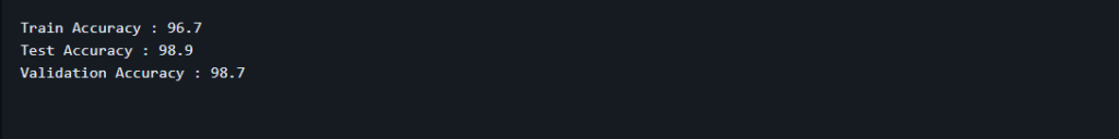
print(
    f"Train Accuracy : {train_acc}\nTest Accuracy : {test_acc}\nValidation Accuracy : {validation_acc}"
)

Output

We evaluated the use of convolutional neural networks to identify plant diseases. We can properly diagnose many plant diseases using deep learning algorithms, allowing farmers to intervene and manage crops more effectively.

To Further Learning:

Research Paper

Research Paper 2

What is the advantage of using convolutional neural networks for plant disease detection?

Convolutional neural networks are very good at identifying small visual clues pointing to plant diseases because they are very good at learning complex photo patterns.

What measures are taken to ensure the model's accuracy and generalization?

Techniques such as dropout regularization and batch normalization are employed within the model architecture to prevent overfitting and promote generalization to unseen data.

Can this model be applied to detect diseases in other types of plants beyond the ones in the provided dataset?

While the model is trained on a specific dataset, it can be adapted to detect diseases in other plants by retraining on relevant data. Transfer learning techniques can also be utilized to fine-tune the model for new tasks.