Wine quality prediction using machine learning
The quality of wine is crucial to both consumers and the wine business. The traditional (professional) method of determining wine quality is very complex. Nowadays, machine learning models are essential instruments for replacing human labor. In this scenario, various features can be used to predict wine quality, but not all will be significant for accurate prediction. As a result, our article focuses on what wine characteristics are critical for achieving a promising outcome. We employed three algorithms (SVM, NB, and ANN) to create a classification model and evaluate relevant features. This work examined two wine-quality datasets: red and white. We used the Pearson coefficient correlation and performance measurement matrices such as accuracy, recall, precision, and f1 score to compare the machine learning algorithms to determine feature importance. A grid search strategy was used to improve model accuracy.
For this project, I used the Red Wine Quality dataset to create multiple classification models that predict whether a given red wine is “good quality” or not. Each wine in this dataset receives a “quality” score between 0 and 10. For this project, I changed the result to a binary output where each wine is either “good quality” (a score of 7 or more) or not (a score of less than 7).
11 input variables determine the quality of wine:
- Fixed acidity
- Volatile acidity
- Citric acid
- Residual sugar
- Chlorides
- Free sulfur dioxide
- Total sulfur dioxide
- Density
- pH
- Sulfates
- Alcohol
Attributes | Description |
fixed acidity | Fixed acids, numeric from 3.8 to 15.9 |
volatile acidity | Volatile acids, numeric from 0.1 to 1.6 |
citric acid | Citric acids, numeric from 0.0 to 1.7 |
residual sugar | residual sugar, numeric from 0.6 to 65.8 |
chlorides | Chloride, numeric from 0.01 to 0.61 |
free sulfur dioxide | Free sulfur dioxide, numeric: from 1 to 289 |
total sulfur dioxide | Total sulfur dioxide, numeric: from 6 to 440 |
density | Density, numeric: from 0.987 to 1.039 |
pH | pH, numeric: from 2.7 to 4.0 |
sulfates | Sulfates, numeric: from 0.2 to 2.0 |
alcohol | Alcohol, numeric: from 8.0 to 14.9 |
quality | Quality, numeric: from 0 to 10, the output target |
Background
A variety of machine learning algorithms are available for the learning process. This section discusses classification algorithms used in wine quality prediction and related research.
Classification algorithm
Naive Bayesian
The naive Bayesian is a simple supervised machine learning classification technique based on Bayes’ theorem. The algorithm assumes that the feature criteria are independent of the class. The naive Bayes algorithm contributes to developing fast machine-learning models capable of making quick predictions. The algorithm uses the likelihood probability to determine whether a specific section has a spot in a particular class.
Support Vector Machine
The most common machine learning algorithm is the support vector machine (SVM). It is a supervised learning model that performs classification and regression tasks. However, it is mainly employed to solve classification problems in machine learning. The SVM method seeks to find the best line or decision boundary to divide an n-dimensional space into classes. So we can quickly place the new data points in the appropriate groupings. The optimal choice boundary is known as a hyperplane. The support vector machine selects the extreme data points that contribute to the formation of the hyperplane. In the diagram above, two distinct groups are classified using the decision boundary or hyperplane. The SVM model applies to both nonlinear and linear data. It uses a nonlinear mapping to turn the primary preparation information into a larger measurement. The model searches for the linearly optimal splitting hyperplane in this new measurement. A hyperplane can divide the data into two classes using proper nonlinear mapping to achieve sufficiently high measurements, and this hyperplane SVM employs support vectors and edges to discover the solution. The SVM model represents the models as a point in space, with the distinct classes separated by a gap to be mapped to ensure that instances are as wide as possible. The model can do nonlinear classification.
Artificial Neural Network
An artificial neural network is a collection of neurons capable of processing information. It has been successfully applied to categorization tasks in various commercial, industrial, and scientific domains. The algorithm model is a connection between neurons linked to the input, hidden, and output layers. The neural network is constant because, even if one of its components fails, it can function in parallel without difficulty.
The implementation of the artificial neural network consists of three layers: input, hidden, and output. The input layer’s function is mapped to the input attribute, which sends feedback to the hidden layer.
Objectives
The project’s objectives are as follows:
- Explaining data sets using Python code.
- To apply various machine learning techniques.
- Experiment with multiple ways to determine which produces the most accuracy.
- To establish which characteristics are most suggestive of high-quality wine.
Wine quality prediction using machine learning with source code
Step 1: Import Libraries
				import numpy as np
import pandas as pd
import seaborn as sns
import matplotlib.pyplot as plt
from sklearn.datasets import load_wine
from sklearn.linear_model import LogisticRegression
from sklearn.svm import SVC
from sklearn.neighbors import KNeighborsClassifier
from sklearn.neural_network import MLPClassifier
from sklearn.ensemble import RandomForestClassifier
from sklearn.preprocessing import StandardScaler, LabelEncoder
from sklearn.model_selection import train_test_split
from sklearn.metrics import confusion_matrix, classification_report,accuracy_score
import warnings
warnings.filterwarnings("ignore")
Step 2: Reading Data
				import wine dataset
wine = datasets.load_wine()
# np.c_ is the numpy concatenate function
wine_df = pd.DataFrame(data= np.c_[wine['data'], wine['target']],
columns= wine['feature_names'] + ['target'])
wine_df.head()
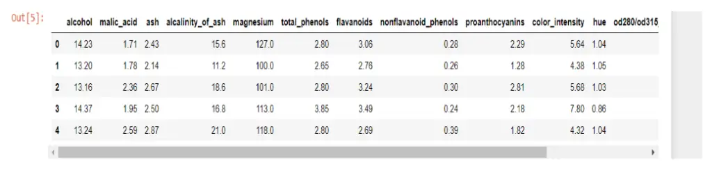
There are 1599 rows and 12 columns. The data was clean in the first five rows, but I wanted to double-check that there were no missing values.
Step 3: Array
Step 4: Missing Values
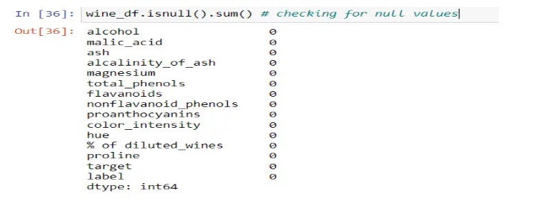
This dataset is ideal for beginners. I did not have to deal with missing values; there wasn’t much room for feature engineering with these variables. Next, I wanted to investigate my data further.
Step 5: Exploring Variables
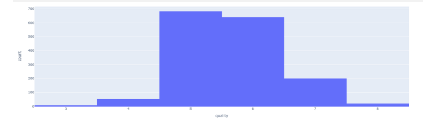
Histogram for ‘quality’ variable
First, I wanted to look at the distribution of the quality variable. I needed to ensure that my dataset contained sufficient ‘good quality’ wines; you’ll see how I defined ‘good quality’ later. The datasets show an uneven distribution of red and white wine, with the two classifications not evenly represented. This unbalanced data can cause overfitting and underfitting algorithms. There are 681 examples of the highest grade class 5 red wine and 2198 instances of the highest quality class 6 white wine. Both datasets are imbalanced, with cases ranging from 5 in the minority class to 681 in red wine and 6 in the minority class to 2198 in the majority class. The most outstanding quality scores are rarely associated with the middle class. Resampling can overcome this problem by adding copies of examples from the under-represented class rather than unnaturally creating such instances (over-sampling) or deleting them from the over-represented class (under-sampling). Unless you have a lot of data, it is an excellent idea to oversample. However, over-sampling has some disadvantages: it increases the number of examples in the dataset, which increases the processing time required to create the model. When the extremes are taken into account, oversampling might result in overfitting. Therefore, resampling is preferred.
				fig = px.histogram(df,x='quality')
fig.show()
Step 6: Correlation Matrix
Next, I wanted to check the correlations between the variables I was working with. This allows me to comprehend the relationships between my variables quickly.
Immediately, some variables are substantially connected with quality. These factors are likely the most essential features in our machine learning model, but we will look into that later.
To better understand the qualities and investigate the correlation between them. We employ Pearson coefficient correlation matrices to determine the correlation between the features.
				plt.figure(figsize=(15,10))
sns.heatmap(wine_df.corr(),annot=True)
plt.show()
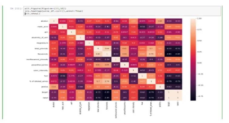
For the above screen, We ranked the features ‘alcohol,’ ‘volatile acidity,’ ‘sulphates,’ ‘citric acid,’ ‘total sulfur dioxide,’ ‘density,’ ‘chlorides,’ ‘fixed acidity,’ ‘pH,’ ‘free sulfur dioxide,’ and residual sugar’ based on their high correlation values to the quality class. Similarly, from Figure 6’s white wine correlation matrix, we ranked the features according to their high correlation values to the quality class, such as ‘alcohol,’ ‘density,’ ‘chlorides,’ ‘volatile acidity,’ ‘total sulfur dioxide,’ ‘fixed acidity,’ ‘pH,’ ‘residual sugar,’ ‘sulfates,’ ‘citric acid,’ and ‘free sulfur dioxide.’
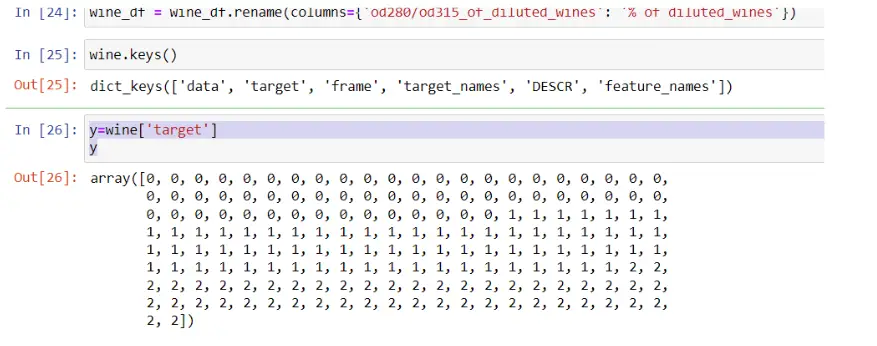
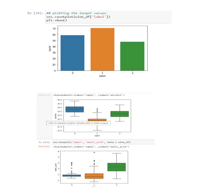
Step 7: Plotting target values
Step 8: Convert to a Classification Problem
Back to my objective, I wanted to compare the effectiveness of various categorization techniques, so I changed the output variable to a binary output.
For this challenge, I defined ‘excellent quality’ as a bottle of wine with a quality score of 7 or higher and ‘poor quality’ as a bottle with a score of less than 7.
After converting the output variable to binary, I split the feature variables (X) and target variable (y) into distinct data frames.
				# Create Classification version of target variable
df['goodquality'] = [1 if x >= 7 else 0 for x in df['quality']]# Separate feature variables and target variable
X = df.drop(['quality','goodquality'], axis = 1)
y = df['goodquality']
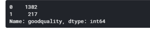
Step 9: Proportion of Good vs Bad Wines
I wanted to make sure that there was a sufficient amount of high-quality wines. Based on the data shown below, it was a reasonable amount. In some cases, resampling may be required if the data is severely skewed, but I assumed it was acceptable.
				# See proportion of good vs bad wines
df['goodquality'].value_counts()
Step 10: Preparing Data for Modelling
At this point, I felt ready to begin preparing the data for modeling. The first thing I did was standardize the dataset. Normalizing the data involves transforming it into a distribution with a mean of 0 and a standard deviation of 1. Standardizing your data is critical for ensuring that the data range is equal.
Consider a dataset with two input features: height (millimeters) and weight (pounds). Because the values of ‘height’ are substantially higher due to measurement, a greater focus will be placed on height than weight, resulting in a bias.
				# Normalize feature variables
from sklearn.preprocessing import StandardScaler
X_features = X
X = StandardScaler().fit_transform(X)
Step 11: Split Data
Next I split the data into a training and test set so that I could cross-validate my models and determine their effectiveness.
				# Splitting the data
from sklearn.model_selection import train_test_split
X_train, X_test, y_train, y_test = train_test_split(X, y, test_size=.25, random_state=0)
Modeling
For this project, I wanted to compare five different machine learning models: decision trees, random forests, AdaBoost, Gradient Boost, and XGBoost. For the purpose of this project, I wanted to compare these models by their accuracy.
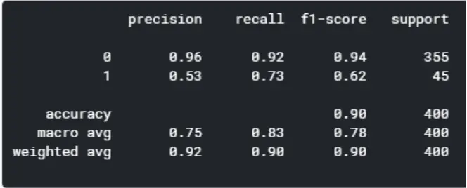
Model 1: Decision Tree
Decision trees are a widely used model in operations research, strategic planning, and machine learning. Each square above represents a node, and the more nodes you have, the more accurate your decision tree will be (in general). The decision tree’s final nodes, when a choice is taken, are known as the leaves of the tree. Decision trees are straightforward to create. However, they need to improve in terms of accuracy.
from sklearn.metrics import classification_report
from sklearn.tree import DecisionTreeClassifiermodel1 = DecisionTreeClassifier(random_state=1)
model1.fit(X_train, y_train)
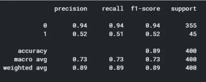
y_pred1 = model1.predict(X_test)print(classification_report(y_test, y_pred1))
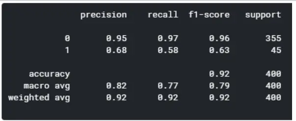
Model 2: Random Forest
Random forests are an approach to group learning based on decision trees. Random forests include building several decision trees from bootstrapped datasets of the original data and randomly selecting a subset of variables at each step of the tree. The model then picks the mode of each decision tree’s predictions. What is the point of this? Using a “majority wins” approach decreases the risk of error from individual trees.
For example, if we design one decision tree, the third one will predict 0. However, if we used the mode of all four decision trees, the anticipated number would be one. This shows the strength of random forests.
				from sklearn.ensemble import RandomForestClassifier
model2 = RandomForestClassifier(random_state=1)
model2.fit(X_train, y_train)
y_pred2 = model2.predict(X_test)print(classification_report(y_test, y_pred2))
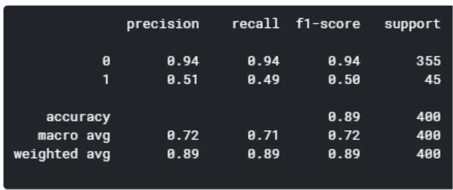
Model 3: AdaBoost
The next following three models are boosting algorithms, which transform weak learners into strong ones. I want to avoid getting sidetracked by explaining the differences between the three, which are extremely extensive and intricate. That being stated, I’ll provide some resources for learning about AdaBoost, Gradient Boosting, and XGBoosting.
				from sklearn.ensemble import AdaBoostClassifier
model3 = AdaBoostClassifier(random_state=1)
model3.fit(X_train, y_train)
y_pred3 = model3.predict(X_test)print(classification_report(y_test, y_pred3))
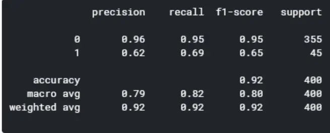
Model 4: XGBoost
				import xgboost as xgb
model5 = xgb.XGBClassifier(random_state=1)
model5.fit(X_train, y_train)
y_pred5 = model5.predict(X_test)print(classification_report(y_test, y_pred5))
Model 5: Gradient Boosting
				from sklearn.ensemble import GradientBoostingClassifier
model4 = GradientBoostingClassifier(random_state=1)
model4.fit(X_train, y_train)
y_pred4 = model4.predict(X_test)print(classification_report(y_test, y_pred4))
By comparing the five models, the random forest and XGBoost seems to yield the highest level of accuracy. However, since XGBoost has a better f1-score for predicting good quality wines (1), I’m concluding that the XGBoost is the winner of the five models.
Feature Importance
I’ve graphed the feature importance using the Random Forest and XGBoost models. While they differ significantly, the top three characteristics remain the same: alcohol, volatile acidity, and sulphates. To compare these characteristics in greater detail, I divided the dataset into high and bad quality, as shown below in the graphs. The applicability of the factors was identified, and the first ten features were chosen from both datasets, with the last feature being omitted. The above red and white wine performance analyses reveal that the performance is accurate.
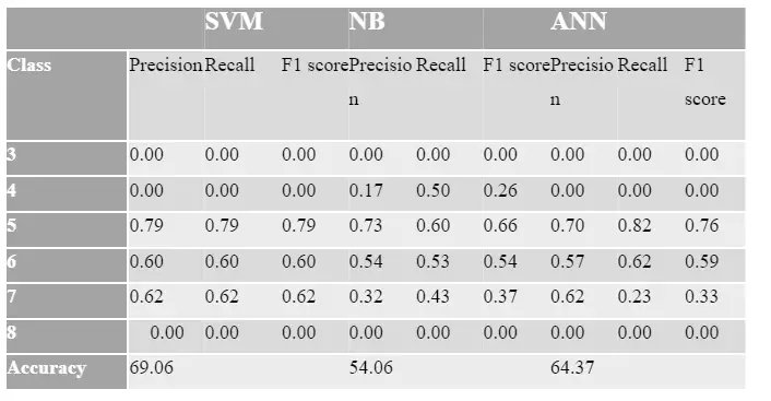
To begin, these chosen features were applied to the unbalanced classes, and the prediction model’s performance in terms of accuracy, precision, recall, and F1 score was examined.
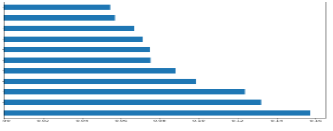
Via Random Forest
				feat_importances = pd.Series(model2.feature_importances_, index=X_features.columns)
feat_importances.nlargest(25).plot(kind='barh',figsize=(10,10))
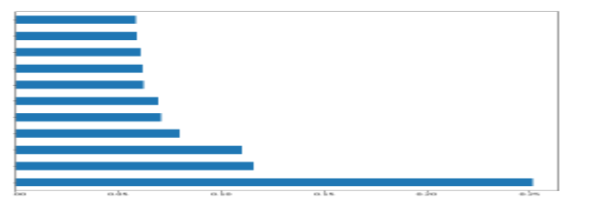
via XGBoost
				feat_importances = pd.Series(model5.feature_importances_, index=X_features.columns)
feat_importances.nlargest(25).plot(kind='barh',figsize=(10,10))
Evaluation
The performance measurement is calculated and evaluate the techniques to detect the effectiveness and efficiency of the model. There are four ways to check the predictions are correct or incorrect:
- True Positive: Number of samples that are predicted to be positive which are truly positive.
- False Positive: Number of samples that are predicted to be positive which are truly negative.
- False Negative: Number of samples that are predicted to be negative which are truly positive.
- True Negative: Number of samples that are predicted to be negative which are truly negative.
Below listed techniques, we use for the evaluation of the model.
1. Accuracy – Accuracy is defined as the ratio of correctly predicted observation to the total observation. The accuracy can be calculated easily by dividing the number of correct predictions by the total number of prediction.
Accuracy= True Positive +True Negative/True Positive + False Positive + False Negative + True Negative
2. Precision – Precision is defined as the ratio of correctly predicted positive observations to the total predicted positive observations.
Precision = True Positive/True Positive + False Positive
4. Recall – Recall is defined as the ratio of correctly predicted positive observations to all observations in the actual class. The recall is also known as the True Positive rate calculated as,
Recall =True Positive/True Positive + False Negative
5. F1 Score – F1 score is the weighted average of precision and recall. The f1 score is used to measure the test accuracy of the model. F1 score is calculated by multiplying the recall and precision is divided by the recall and precision, and the result is calculated by multiplying two.
F1 score = 2 ∗Recall ∗ Precision Recall + Precision
Accuracy is the most widely used evaluation metric for most traditional applications. But the accuracy rate is not suitable for evaluating imbalanced data sets, because many experts have observed that for extremely skewed class distributions, the recall rate for minority classes is typically 0, which means that no classification rules are generated for the minority class. Using the terminology in information retrieval, the precision and recall of the minority categories are much lower than the majority class. Accuracy gives more weight to the majority class than to the minority class, this makes it challenging for the classifier to implement well in the minority class.
Additional measures are increasingly being used for this purpose. The F1 score is a popular metric for estimating the imbalanced class problem (Estabrooks & Japkowicz, 2001). The F1 score combines two matrices: precision and recall. Precision refers to how accurately the model predicted a specific class, whereas recall refers to the number of misplaced instances that were incorrectly classified. Because numerous classes have different F1 scores. We use the unweighted mean of the F1 scores for our final scoring. We want our models to be optimized to classify instances that are in the minority, such as wine quality of 3, 8, or 9, just as well as the other attributes that are represented in a higher number.
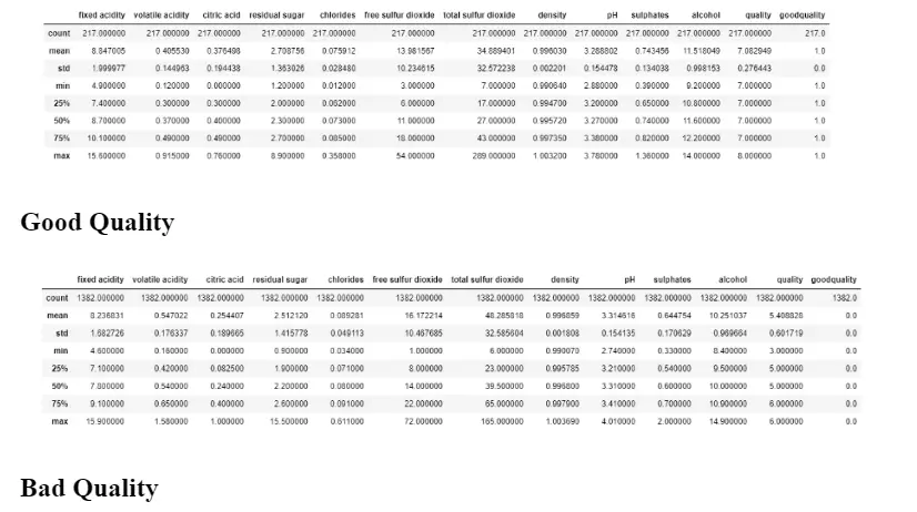
Comparing the Top 4 Features
				# Filtering df for only good quality
df_temp = df[df['goodquality']==1]
df_temp.describe()# Filtering df for only bad quality
df_temp2 = df[df['goodquality']==0]
df_temp2.describe()
Conclusion
We use correlation matrices to calculate the relationship between all features, as seen in red wine correlation matrices. We then ranked the features of these unbalancing and balancing. We achieved higher performance results on the balanced class for all models.
Based on a solid link with the quality attribute. The study of feature groups from left to right is carried out, and the first ten features are chosen, while the final feature is rejected because there is no improvement, and it reduces the model’s performance. The final model implementation does not include the residual sugar’ feature from the red wine datasets and the ‘free sulfur dioxide feature from the white wine datasets. After evaluating the importance of the features, we begin implementing the model. To estimate the model’s performance, we applied it to the original data (unbalanced class) and then to the balanced class, balancing each class. The prediction model’s accuracy, precision, recall, and f1 score are evaluated, as well as the performance analysis results for imbalanced classes for each model. Looking at the specifics, we can see that good quality wines have greater alcohol levels on average, lower volatile acidity on average, higher levels of sulfates on average, and higher levels of residual sugar on average.
The accuracy of machine learning predictions depends on the quality and quantity of the data used for training. With robust datasets and advanced algorithms, predictions can be remarkably accurate, providing valuable insights for winemakers.
Winemakers can benefit from machine learning by gaining valuable insights into grape quality, optimal harvesting times, and personalized recommendations for consumers. It enhances precision viticulture, streamlining the winemaking process and ultimately contributing to the production of higher-quality wines.
Machine learning is a beautiful technology, but it has limitations. Dealing with varied grape types and unexpected weather patterns presents obstacles. However, technological improvements aim to address these limits and improve machine learning skills in the wine sector.

Final Year Projects

Data Science Projects

Blockchain Projects

Python Projects

Cyber Security Projects

Web dev Projects

IOT Projects

C++ Projects
-
Where Do YouTubers Get Their Music?
-
Top 20 Machine Learning Project Ideas for Final Years with Code
-
Why Creators Choose YouTube: Exploring the Four Key Reasons
-
10 Advance Final Year Project Ideas with Source Code
-
10 Deep Learning Projects for Final Year in 2024
-
Realtime Object Detection
-
AI Music Composer project with source code
-
30 Final Year Project Ideas for IT Students
-
E Commerce sales forecasting using machine learning
-
Stock market Price Prediction using machine learning
-
c++ Projects for beginners
-
Python Projects For Final Year Students With Source Code
-
20 Exiciting Cyber Security Final Year Projects
-
10 Web Development Projects for beginners
-
Top 10 Best JAVA Final Year Projects
-
Fake news detection using machine learning source code
-
C++ Projects with Source Code
-
15 Exciting Blockchain Project Ideas with Source Code
-
Artificial Intelligence Projects For Final Year
-
Best 21 Projects Using HTML, CSS, Javascript With Source Code
-
Hand Gesture Recognition in python
-
Credit Card Fraud detection using machine learning
-
How to Download image in HTML
-
How to Host HTML website for free?
-
Hate Speech Detection Using Machine Learning
-
10 advanced JavaScript project ideas for experts in 2024
-
Python Projects For Beginners with Source Code
-
Best Machine Learning Final Year Project
-
20 Advance IOT Projects For Final Year in 2024
-
Top 7 Cybersecurity Final Year Projects in 2024
-
Data Science Projects with Source Code
-
Plant Disease Detection using Machine Learning
-
Ethical Hacking Projects
-
10 Exciting C++ projects with source code in 2024
-
Artificial Intelligence Projects for the Final Year
-
Best 13 IOT Project Ideas For Final Year Students
-
Top 13 IOT Projects With Source Code
-
portfolio website using javascript
-
Phishing website detection using Machine Learning with Source Code
-
17 Easy Blockchain Projects For Beginners
-
10 Exciting Next.jS Project Ideas
-
Fabric Defect Detection
-
Heart Disease Prediction Using Machine Learning
-
How to Change Color of Text in JavaScript
-
Wine Quality Prediction Using Machine Learning
-
Diabetes Prediction Using Machine Learning
-
10 Final Year Projects For Computer Science With Source Code
-
Car Price Prediction Using Machine Learning
-
10 TypeScript Projects With Source Code
-
Step-By-Step Complete Guide Of Freelance Visa Abu Dhabi In 2024
